
Experimental stations
Exploring the Intensity of Radiation
Changing the distance from the radioactive source
In this FAR Lab experiment you will monitor and plot the number of counts recorded by a Geiger counter as you increase the distance from the source.
In the Turntable experiment, the radiation came from four real radioactive samples; an alpha source, a beta source, a gamma source and an unknown source (which you should have worked out!).
In this experiment it doesn’t matter what kind of radiation it is. All that matters is how the number of counts changes as you get further away from the detector.
We know that radioactive emissions are potentially very harmful to humans. If there is no barrier between us and a radioactive source, how far away do we need to be to be safe?
-
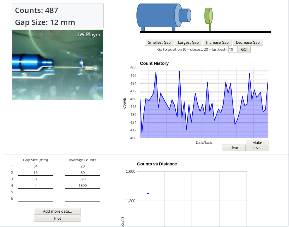
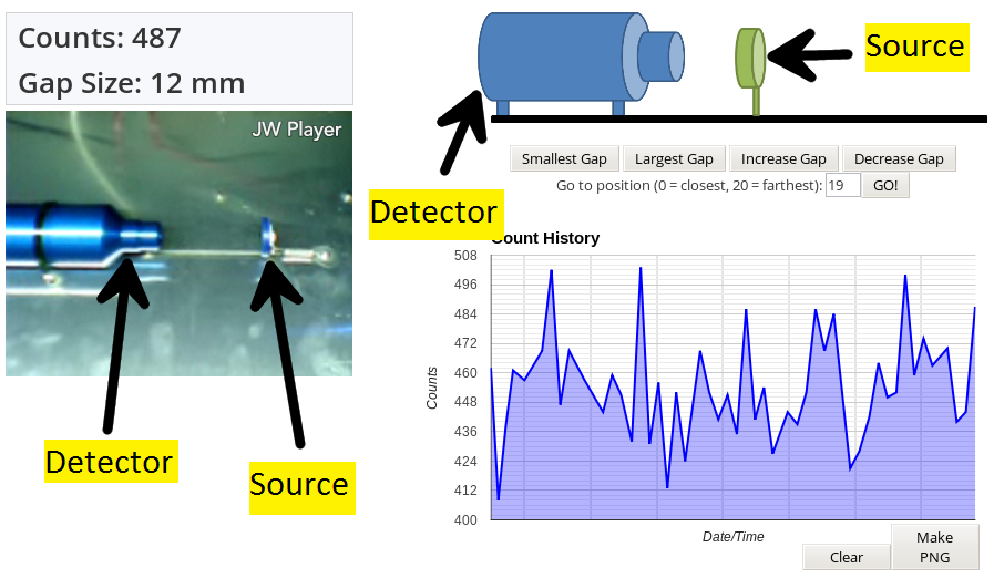
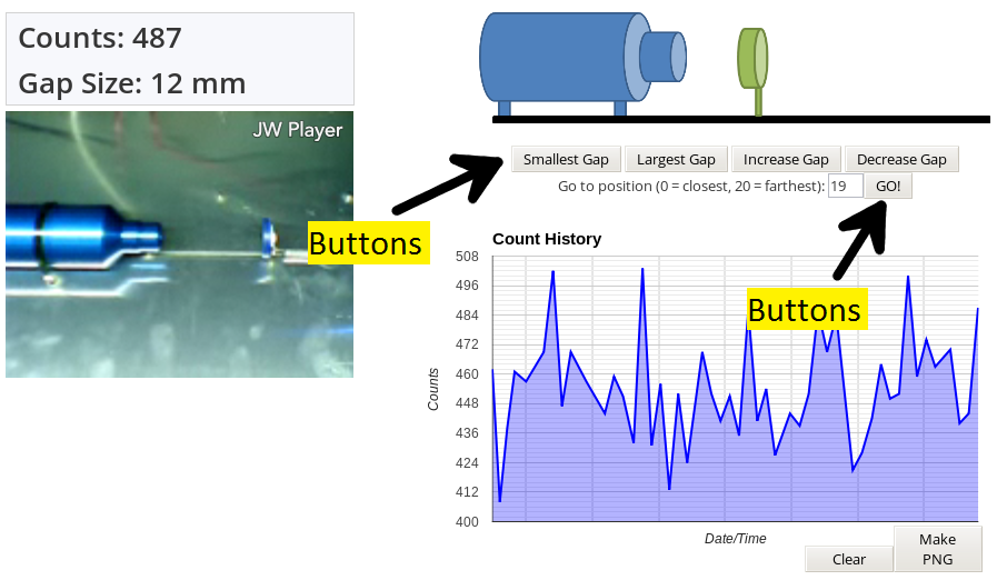
In the middle of the screen there is a diagram showing the radioactive source (Green) and detector (Blue). The detector and source can also be seen in the video feed to the left . Underneath the diagram, there are buttons labelled “Smallest Gap”, “Largest Gap”, “Increase Gap” and “Decrease Gap”.
 Click to enlarge
-
The buttons help you move the source to 11 different positions ranging from 20 mm to 90 mm from the detector. If you want to move a large distance in a short amount of time, you can type in a number from 0 to 10 in the text box and click the “GO!” button. Clicking the “Increase Gap” and “Decrease Gap” buttons moves the source by a small amount.
 Click to enlarge
What we’re most interested in is the effect distance has on the “Counts” at the detector. We are going to plot a graph of counts versus distance. What do you think your graph will look like? A curve? A straight line?
Plotting your graph
Method:
- Make sure that your source is as close to the detector as possible. You can do this by clicking the “Smallest Gap” button underneath the diagram (Check that the source is right up against the detector in the video feed on the left). The “Gap Size” should say 20 mm.
- Wait for a few seconds and then take at least five recordings of the “Counts” and make a note in your lab books OR
- Use the “Count History” graph next to the video screen to record the counts. Wait for your Count History graph to record at least 15 seconds of data then click the “Make PNG” button under the graph. A snapshot of the graph at that point will open in a new window.
- Find the average by adding up your recordings and dividing by 5 (if you did step 2 and wrote down 5 numbers) OR by ruling a straight line horizontally across your Count History graph where you think the middle value is (if you did step 3).
- Once you find the average you can start filling in the table below the video feed. The number for the “Gap Size” is above the video feed while the “Average Counts” is the average you just found.
- Repeat this process for several different distances and keep filling in the table. Ask your teacher how many distances you need to do.
- When you have enough values, you can see what your graph looks like by clicking the “Plot” button. Before you click Plot ask your partner what they think the graph will look like! What do you think?
- Download a copy of your data using the Data Browser.
Question:
- What shape did the graph have? Was this what you expected?
- If you double the distance away from the source what happens to the counts?
- Do you think that a different radiation source (alpha/beta/gamma) would produce a different graph? If so, how? Would the shape be different?
Can you explain why the Counts decrease in the way you have observed?